Physics Based Differentiable Rendering: Preliminaries

Introduction

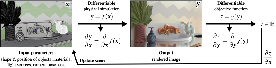
Differentiable rendering is the inverse problem of traditional rendering. Instead of rendering the image from given scene parameters, differentiable rendering trying to recover scene parameter from a given image. To do this, a common idea is using gradient based optimization methods like SGD, Adam, etc. An important part of gradient based optimization is calculating the derivative of the render result w.r.t. certain scene parameters.

In traditional physics based rendering, we have various methods like path tracing, bidirectional path tracing, photon mapping, etc to achieve great render result. These methods are all trying to solve the rendering equation described as below:

$$
L_o(\pmb x,\omega_o,\lambda,t)=L_e(\pmb x,\omega_o,\lambda,t)+\int_\Omega f_r(\pmb x,\omega_i,\omega_o,\lambda,t)L_i(\pmb x,\omega_i,\lambda,t)(\omega_i\cdot\pmb n)\mathrm d\omega_i
$$

Now we want to calculate the the derivative of the render result w.r.t. certain scene parameters like $\pi$, a straight forward way to solving the derivative of the rendering equation:

$$
\frac{\partial}{\partial\pi}L_o(\pmb x,\omega_o,\lambda,t)=\frac{\partial}{\partial\pi}L_e(\pmb x,\omega_o,\lambda,t)+\frac{\partial}{\partial\pi}\int_\Omega f_r(\pmb x,\omega_i,\omega_o,\lambda,t)L_i(\pmb x,\omega_i,\lambda,t)(\omega_i\cdot\pmb n)\mathrm d\omega_i
$$

In computer algebra, we can use automatic differentiation to solving the derivative of a computing process w.r.t. some parameters. In most case, automatic differentiation is quite well. However, using automatic differentiation requires the process to be smooth. In rendering task, many situations can break the smoothing condition, like geometry edges, object silhouettes, etc. Therefore, we need some special methods to handle this failed cases. Calculating derivative of the rendering equation correctly and fast is one of the most important parts of differentiable rendering.

Another important part of differentiable rendering is handle complex light transportation. We already have many light transport theorem to help us handle complex light transportation rendering like caustics, dispersion, subsurface scattering, volumetric rendering, etc. Simply using general differentiable rendering methods on these tasks may not always work well. Many researchers are working on this topic as well.

Since we have some basic methods to deal with differentiable rendering problem, what can it do next? A common application of differentiable rendering is scene reconstruction. Using the derivative of the rendering result w.r.t. some parameters waiting to be optimized, we can easily do some reconstruction tasks, like reconstructing geometry (optimizing vertex position/SDF parameters), reconstructing material (optimizing BSDF parameters), reconstructing light condition (optimizing emissive parameters), etc. Due to the power of realistic rendering, physics based differentiable rendering can do somthing that other reconstruction methods can’t, like taking full use of indirect illumination.

Reynolds Transport Theorem

As we describe before, calculating the derivative of the rendering equation is solving:

Assuming $I=\int_{\mathcal X} f(x,\Theta)\mathrm dx=\int_{\Omega} f_r(\pmb x,\omega_i,\omega_o,\lambda,t)L_i(\pmb x,\omega_i,\lambda,t)(\omega_i\cdot\pmb n)\mathrm d\omega_i$
If $f(x,\Theta)$ is smooth, we can easily apply:

$$
\frac{\partial}{\partial\pi}\int_{\mathcal X} f(x,\Theta)\mathrm dx=\int_{\mathcal X}\frac{\partial}{\partial \pi}f(x,\Theta)\mathrm dx
$$
However, $f(x,\Theta)$ is not always smooth due to visibility, etc. In these cases, we can’t straightly calculate the derivative of $f(x,\Theta)$.

Consider a simple case in 1D:

$$
I=\int_a^bf(x,\pi)\mathrm dx
$$
Where $b\leq x\leq a$, and $f(x)$ has discontinuties at $p_1(\pi),p_2(\pi),\cdots,p_n(\pi)$. Therefore,

$$
\frac{\partial I}{\partial\pi}\neq \int_a^b\frac{\partial}{\partial\pi}f(x,\pi)\mathrm dx
$$
A trick to solve this problem is moving all discontinuties to the integral boundary, like:

$$
I=\int_a^{p_1(\pi)}f(x,\pi)\mathrm dx+
\int_{p_1(\pi)}^{p_2(\pi)}f(x,\pi)\mathrm dx+\cdots+
\int_{p_n(\pi)}^bf(x,\pi)\mathrm dx
$$
In this case, $f(x)$ become smooth in $[a,p_1(\pi)]$, $[p_1(\pi),p_2(\pi)]$, $\cdots$, $[p_n(\pi), b]$.

Based on Leibiniz integral rule, we know that

$$
\frac{\partial}{\partial \pi}\int_{p_i(\pi)}^{p_{i+1}(\pi)}f(x,\pi)\mathrm dx=f^-(p_{i+1}(\pi))\cdot\frac{\mathrm d}{\mathrm d\pi}p_{i+1}(\pi)-f^+(p_{i}(\pi))\cdot\frac{\mathrm d}{\mathrm d\pi}p_{i}(\pi)+\int_{p_i(\pi)}^{p_{i+1}(\pi)}\frac{\partial}{\partial \pi}f(x,\pi)\mathrm dx
$$
Assuming $a=p_0(\pi)$, $b=p_{n+1}(\pi)$, $\Delta f_i=f^-(p_{i+1}(\pi))\cdot\frac{\mathrm d}{\mathrm d\pi}p_{i+1}(\pi)-f^+(p_{i}(\pi))\cdot\frac{\mathrm d}{\mathrm d\pi}p_{i}(\pi)$

$$
\begin{aligned}
\frac{\partial I}{\partial \pi}&=\sum_{i=0}^{n+1}\left(f^-(p_{i+1}(\pi))\cdot\frac{\mathrm d}{\mathrm d\pi}p_{i+1}(\pi)-f^+(p_{i}(\pi))\cdot\frac{\mathrm d}{\mathrm d\pi}p_{i}(\pi)+\int_{p_i(\pi)}^{p_{i+1}(\pi)}\frac{\partial}{\partial \pi}f(x,\pi)\mathrm dx\right)\\
&=\sum_{i=0}^{n+1}\Delta f_i +\sum_{i=0}^{n+1}\int_{p_i(\pi)}^{p_{i+1}(\pi)}\frac{\partial}{\partial \pi}f(x,\pi)\mathrm dx
\end{aligned}
$$
We can see original equation is divided into two parts: interior term $\sum_{i=0}^{n+1}\int_{p_i(\pi)}^{p_{i+1}(\pi)}\frac{\partial}{\partial \pi}f(x,\pi)\mathrm dx$ and boundary term $\sum_{i=0}^{n+1}\Delta f_i$

We can generalize above deduction to three-dimensions to become Reynolds Transport theorem:

$$
\frac{\partial}{\partial t}\int_{\Omega(t)}\pmb f\mathrm dV=\int_{\Omega(t)}\frac{\partial\pmb f}{\partial t}\mathrm dV+\int_{\partial\Omega(t)}(\pmb v_b\cdot\pmb n)\pmb f\mathrm dA
$$

Interior term: $\int_{\Omega(t)}\frac{\partial\pmb f}{\partial t}\mathrm dV$
Boundary term: $\int_{\partial\Omega(t)}(\pmb v_b\cdot\pmb n)\pmb f\mathrm dA$
$\pmb n(\pmb x,t)$ is the outward-pointing unit normal vector, $\pmb x$ is a point in the region and is the variable of integration
$\mathrm dV$ and $\mathrm dA$ are volume and surface elements at $\pmb x$
$v_b(\pmb x,t)$ is the velocity of the area element

In differentiable rendering, interior term can be easily calculated by automatic differentiation, and the boundary term is not that easy. Most of the research focus on solving boundary term accurately and quickly, which I will write a series of notes for explaining the details.

Automatic Differentiation

The key idea of automatic differentiation is the chain rule:

$$
\frac{\partial z}{\partial \pmb x}=\frac{\partial z}{\partial \pmb y}\cdot\frac{\partial \pmb y}{\partial \pmb x}
$$

Single variable case :

$$
\begin{aligned}
y=f(x)\\\\
z=g(y)
\end{aligned}
$$

graph LR 
	X-->Y 
	Y-->Z

$$
\begin{matrix}
\dfrac{\mathrm dy}{\mathrm dx}&\dfrac{\mathrm dz}{\mathrm dy}
\end{matrix}
$$

Multiple variable case:

$$
\begin{aligned}
y&=f(x_0, x_1)\\\\
z&=g(y)
\end{aligned}
$$

graph LR
    X0-->Y
    X1-->Y
    Y-->Z

$$
\begin{aligned}
\frac{\partial z}{\partial x_0}&=\frac{\partial z}{\partial y}\frac{\partial y}{\partial x_0}\\\\
\frac{\partial z}{\partial x_1}&=\frac{\partial z}{\partial y}\frac{\partial y}{\partial x_1}
\end{aligned}
$$

We can see the result $\partial z/\partial y$ can be reused. Therefore, for a complex computing process, we can construct a compute graph, searching for the best path to calculate the derivative using chain rule.

There are two ways to execute automatic differentiation: forward mode and reverse mode

Forward Mode

graph LR
    W0-->X
    W1-->X
    W2-->X
    W0-->Y0
    X-->Y0
    X-->Y1
    Y0-->Z
    Y1-->Z

Forward mode automatic differentiation start from the beginning of the compute graph, and propagate the derivative forward. Assuming we want to calculate $\partial z/\partial w_0$ form the compute graph above, we do:

$$
\begin{aligned}
W0:&\frac{\partial w_0}{\partial w_0}=1\\\
W1:&\frac{\partial w_1}{\partial w_0}=0\\\
W2:&\frac{\partial w_2}{\partial w_0}=0\\\
X:&\frac{\partial x}{\partial w_0}\\\
Y0:&\frac{\partial y_0}{\partial w_0}=\frac{\partial y_0}{\partial x}\frac{\partial x}{\partial w_0}+\frac{\partial y_0}{\partial w_0}\\\
Y1:&\frac{\partial y_1}{\partial w_0}=\frac{\partial y_1}{\partial x}\frac{\partial x}{\partial w_0}\\\
Z:&\frac{\partial z}{\partial w_0}=\frac{\partial z}{\partial y_0}\frac{\partial y_0}{\partial w_0}+\frac{\partial z}{\partial y_1}\frac{\partial y_1}{\partial w_0}
\end{aligned}
$$

Reverse Mode

graph LR
    W0-->X
    W1-->X
    W2-->X
    W0-->Y0
    X-->Y0
    X-->Y1
    Y0-->Z
    Y1-->Z

Reverse mode automatic differentiation start from the end of the compute graph, and propagate the derivative backward. Like the compute graph above, start from $z$, we have:

$$
\begin{aligned}
Y0:&\frac{\partial z}{\partial y_0}\\\\
Y1:&\frac{\partial z}{\partial y_1}\\\\
X:&\frac{\partial z}{\partial x}=\frac{\partial z}{\partial y_0}\frac{\partial y_0}{\partial x}+\frac{\partial z}{\partial y_1}\frac{\partial y_1}{\partial x}\\\\
W0:&\frac{\partial z}{\partial w_0}=\frac{\partial z}{\partial y_0}\frac{\partial y_0}{\partial w_0}+\frac{\partial z}{\partial x}\frac{\partial x}{\partial w_0}\\\\
\cdots
\end{aligned}
$$

In differentiable rendering, reverse mode automatic differentiation is used for optimization and forward mode automatic differentiation is used for gradient visualization.

Reference

TODO

Physics Based Differentiable Rendering: Preliminaries

Introduction

Reynolds Transport Theorem

Automatic Differentiation

Reference

Reasearcher & Lab

Course

Tool

Paper