ExtraNet: Real-time Extrapolated Rendering for Low-latency Temporal Supersampling
Abstract
Real-time Rendering
- Frame rate
- Latency
Spatial Super Sampling: DLSS
- Decreasing the rendering time of each frame by rendering at a lower resolution
Temporal Super Sampling
- Producing more frames on the fly
- Problems:
- It’s own computational cost
- The latency introduced by interpolating frames from the future
ExtraNet
An efficient neural network that predicts accurate shading results on an extrapolated frame, to minimize both the performance overhead and the latency
Rendered auxiliary geometry buffers of the extrapolated frame & Temporally reliable motion vectors
Train to perform two tasks:
- Irradiance in-painting for regions that cannot find historical correspondences
- Accurate ghosting-free shading prediction for regions where temporal information is available
A robust hole-marking strategy to automate the classification of these tasks
The data generation from a series of high-quality production-ready scenes
1. Introduction
Some techniques to increase the rendering performance
Leveraging the temporal coherency between frames: Reduces the sampling rate at each individual frame, and rely on temporal reprojections to combine samples taken over multiple frames to reconstruct a high quality image (Still performing spatial upsampling / reconstruction, with a virtually higher sampling rate acquired temporally to speed up the generation of the current frame of interest)
- TAA (Temporal Anti-Aliasing)
- TAAU (Temporal Anti-Aliasing Upsample)
- DLSS (Deep Learning Super Sampling)
- Ray Tracing Denoising
Limitation of current work
- Frame Interpolation: only when the next frame has been fully rendered, their algorithms can start to work to interpolate one or more frames in between
- Performance: generating a new frame is already more expensive than a full rendering of it
- Situation: more information can be used in rendered scene, like G-buffers
Contribution
- A new temporally interleaved real-time rendering and extrapolation architecture that can nearly double the frame rate without introducing additional latency.
- A novel neural network architecture that leverages G-buffers and temporal motion (computed both from consecutive frames and temporally reliable motion vectors) to perform the extrapolation as a shading prediction task.
- A lightweight design that incurs low performance overhead (around 8 milliseconds per frame at 720P) but results in high quality and smoothly extrapolated frames.
2. Related work and background
2.1. Temporal Reconstruction
- Rely on temporal motion vectors
- Temporal reconstruction methods reduce the samples taken at each individual frame, and reproject samples over the course of multiple frames using backward motion vectors to reconstruct a high quality image
- In their paper
- Leverage temporal motion vectors to reproject shading of the previous rendered frames to the extrapolated frames
- But they do not have any samples in the extrapolated frames, unlike temporal reconstruction
Motion Vectors
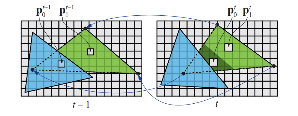
$$
\pmb p_0^{t}=\pmb P^t\pmb M^t\pmb V^t \pmb s_0
$$
$$
\pmb p_0^{t-1}=\pmb P^{t-1}\pmb M^{t-1}\pmb V^{t-1}\pmb s_0
$$
Store screen space motion vectors => Velocity Buffer
vertex shader:
1 | uniform mat4 uModelViewProjectionMat; |
fragment shader:
1 | smooth in vec4 vPosition; |
2.2. Texture In-painting
Using backward motion vectors to reproject shading from previous frame is that disoccluded regions will not contain any valid information in the previous frame, resulting in “holes” in the reprojected image
Some work:
- Convolution
- Deep learning
- Resort to a two-stage prediction strategy to separately predict missing textures in a step-by-step manner
Limitation
- Not designed specifically for real-time rendering
- Perform the in-painting task completely on single images without temporal information and G-buffers
- The running time of some methods are in the order of seconds, which are not suitable in our real-time extrapolation task
2.3. Image Warping
- Realized by forward scattering or backward gathering, according to their data access patterns
- Compared with forward mapping, backward mapping is more appealing in real-time rendering due to its high efficiency
- Although visually plausible contents can be recovered at hole regions after image warping, shadow and highlight movements are almost untouched in these traditional methods, especially those used in the context of frame extrapolation
2.4. Video and Rendering Interpolation
- Interpolation based frame rate upsampling is widely used for temporally upsampling videos, using optical flow of the last couple of frames
- Optical flow is an image based algorithm that often produces inaccurate motion, which will lead to artifacts in the interpolation results
- Uses accurate motion vectors available from the rendering engine, usually rely on image warping techniques to reuse shading information across frames
- Deep learning based video interpolation methods are still time-consuming, thus are not suitable for real-time rendering
3. Motivation and Challenge
3.1. Latency
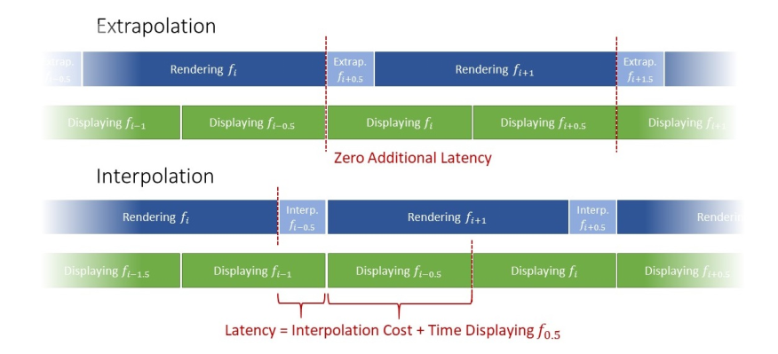
- Interpolation => Produce significant lantency
- Extrapolation => doesn’t introduce any additional latency
3.2. Challenge
Disocclusion
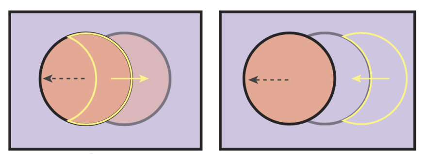
- Backward motion vectors may not always exist
- Traditional motion vectors propose to use the same pixel values from previous frames, resulting in ghosting artifacts in the disoccluded regions
- Occlusion motion vectors alleviates this problem by looking for a nearby similar region in the current frame, then look for the corresponding region from previous frames
- Leverage an in-painting network to reshade the occluded regions using occlusion motion vector
Dynamic changes in shading
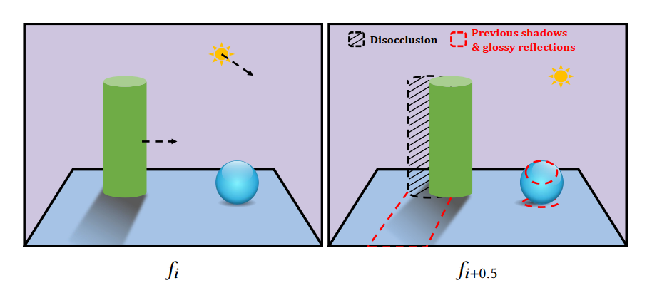
- Dynamic changes in shading over frames, such as moving shadows, parallax motion from reflections and the colors on rotating objects, may change drastically and are thus unknown in the current frame
- Always keep the most recently rendered 3 frames for the network to learn to extrapolate the changes
Other challenges
- Extremely low tolerance towards errors and artifacts
- The inference of the neural network must be (ideally much) faster than the actual rendering process
4. ExtraNet for frame extrapolation
Design and train a deep neural network, namely ExtraNet, to predict a new frame from some historical frames and the G-buffers of the extrapolated frame.
- Considering that disoccluded regions of the extrapolated frame lack shading information but reliable and cheap G-buffers are available, we construct an In-painting Network to reshade the disoccluded regions with the help of occlusion motion vectors and those G-buffers
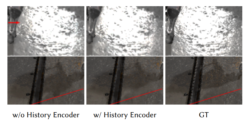
- In contrast to the general image in-painting task, regions that are not disoccluded may also contain invalid pixels attributing to dynamic shading changes in the scene. To tackle this issue, we design a History Encoder, an additional convolutional neural network, to extract necessary information from historical frames
- To meet the requirement of high inference speed which is critical to real-time rendering, adopting lightweight gated convolutions in the In-painting Network.
4.1. Problem Formulation
- Frame $i$: Denoting the current frame rendered by the graphics engine
- Frame $i+0.5$: Next frame the network will predict
- Two historical frames including frame $i-1$ and $i-2$ and the corresponding G-buffers
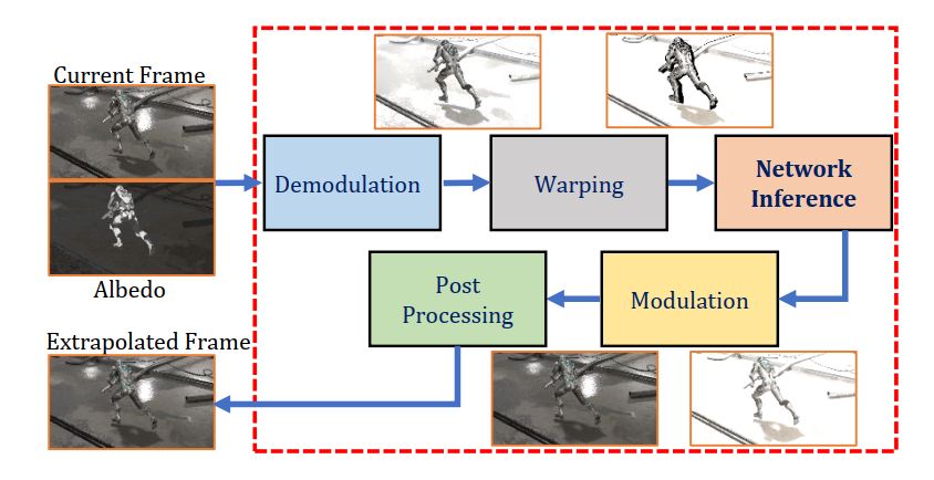
Pipeline:
- Demodulation: Dividing by the albedo to acquire texture-free irradiance
- Warp the demodulated frame using both traditional backward motion vectors and occlusion motion vectors
- The warping operation probably incurs holes in the frame. Using In-painting network to fill the frame
- Modulation: multiplying by the albedo to re-acquire textured shading
- Apply regular post-processing(tone mapping ,TAA…)
4.2. Motion Vectors and Image Warping
Instead of computing a zero motion vector in disoccluded regions as the traditional backward motion vector does, occlusion motion vector computes the motion vector in disoccluded regions as the motion vector of the foreground in the previous frame
4.3. Network Architecture
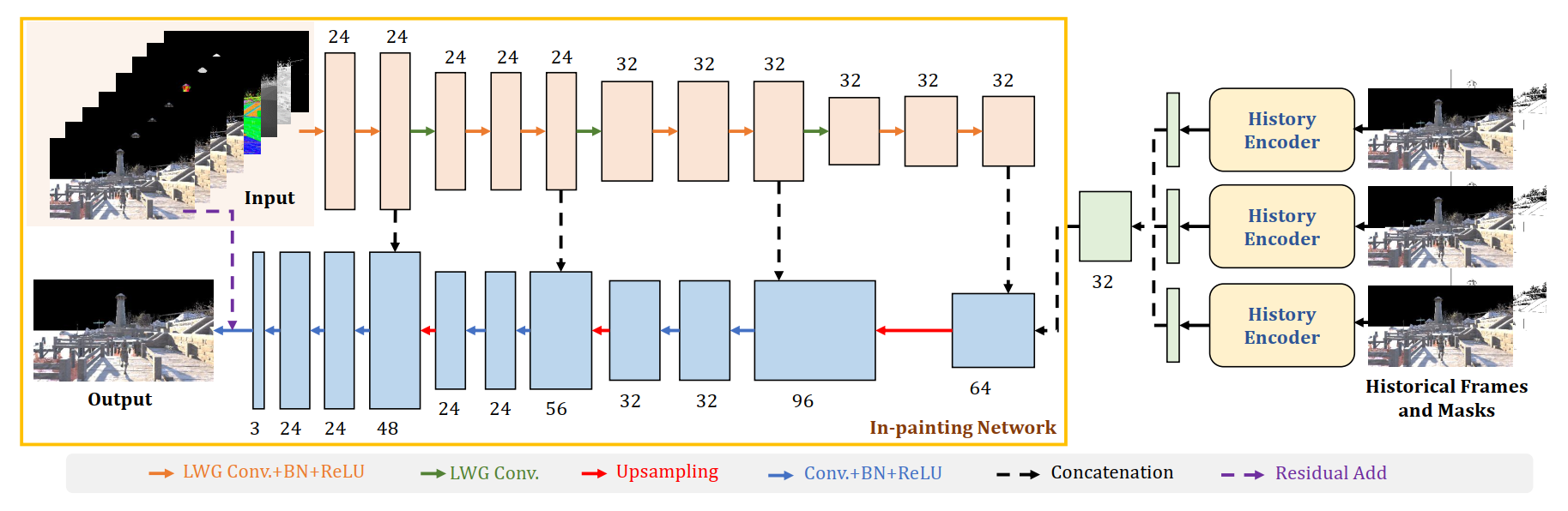
Similar structure with U-NET
Adopt gated convolutions
$$
\pmb M=\mathrm{Conv}(\pmb W_m, \pmb X)
$$$$
\pmb F=\mathrm{Conv}(\pmb W_f,\pmb X)
$$$$
\pmb O=\sigma(\pmb M)\odot \pmb F
$$- $\pmb X$: Input feature map
- $\pmb W_m$ and $\pmb W_f$: Two trainable filters
- $\odot$ : Element-wise multiplication
- $\sigma(\cdot)$: Sigmoid activation
Gated convolutions increase the inference time
- Resort to a light-weight variant of gated convolution by making $\pmb M$ a single-channel mask
- Not use any gated convolution in the upsampling stage
- Assume all holes have already been filled in the downsampling stage
Use a residual learning strategy in our pipeline by adding the predicted image of our network with the input image warped by traditional backward motion vectors
- This stabilizes the training process
4.4. History Encoder
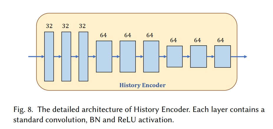
Input: Warped images of the current frame $i$ and its two past frames including frame $i-1$ and frame $i-2$
- Warp frames $i-1$ and $i-2$: accumulate the motion vectors
- Invalid pixels should be marked for these frames
Structure: Nine $3\times 3$ convolution layers
- Down sample the input
- Shared by different historical frames
Output: Implicitly encode the high-level representations of shadows and shadings in previous frames, are concatenated together and fed into our In-painting Network
Optical flow can be explicitly predicted from several historical frames
- But correct forward optical flow is difficult to acquire in the frame extrapolation pipeline, since only historical frames are available
- Use backward optical flow as an approximation
- Not using it
4.5. Loss Function
Penalizes pixel-wise error between the predicted frame $\pmb P$ and ground-truth frame $\pmb T$
$$
\mathcal L_{l_1}=\frac{1}{n}\sum_i |\pmb P_i - \pmb T_i|
$$
hole-augmented loss: penalize more in the hole regions marked beforehand
$$
\mathcal L_{\mathrm {hole}}=\frac{1}{n}\sum_i |\pmb P_i-\pmb T_i|\odot(1-\pmb m)
$$
- $\pmb m$ is the binary mask fed into network
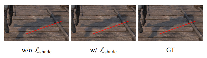
The shading-augmented loss: focuses on handling potential shading changes in the predicted frames
$$
\mathcal L_{\mathrm{shade}}=\frac{1}{k}\sum_{i\in \Phi_{\mathrm{top}-k}}|\pmb P_i-\pmb T_i|
$$
- Shading changes: stem from moving shadows due to dynamic lights and specular reflections
- Considering that shadows and reflections tend to generate large pixel variation among neighboring frames, we select $𝑘$ pixels with top $𝑘$ largest errors from the predicted frame and mark these pixels as potential shading change regions
- $\Phi_{\mathrm{top}-k}$ includes the indices of $k$ pixels with top $k$ largest errors
- Currently, $k$ set to 10% of total pixels number
Final loss function
$$
\mathcal L=\mathcal L_{l_1}+\lambda_{\mathrm{hole}}\mathcal L_{\mathrm{hole}}+\lambda_{\mathrm{shade}}\mathcal L_{\mathrm{shade}}
$$
- $\lambda_{\mathrm{hole}}$ and $\lambda_{\mathrm{shade}}$are weights to balance the influence of the losses, here set to 1
4.6. Training detail
- PyTorch
- Mini-batch SGD and Adam optimizer
- mini-batch size as 8, $\beta_1 = 0.9$ and $\beta_2=0.999$ in Adam optimizer
- default initialization
- applied HDR image: logarithm transformation $y=\log(1+x)$ before feeding images into network
5. Dataset
5.1. Scenes and Buffers

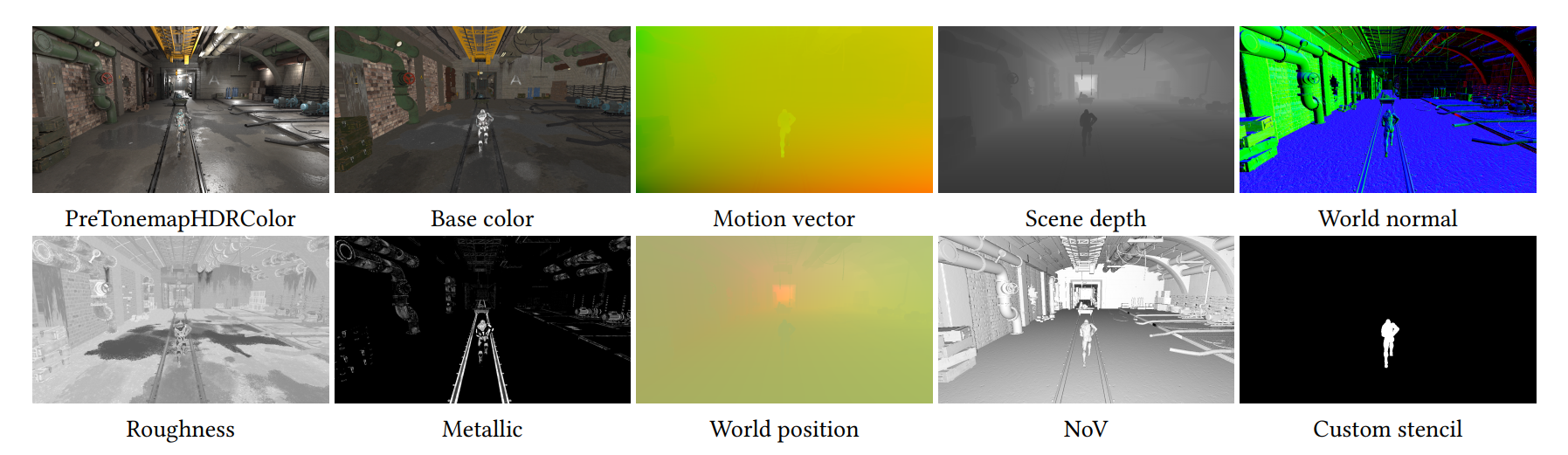
Each dumped frame comprises 10 buffers which can be divided into three categories:
- Actual shading frame before tone mapping (PreTonemapHDRColor) and albedo (Base color) for demodulation
- G-buffers used in our network, including scene depth ($𝑑$, 1channel), world normal ($\pmb n_𝑤$, 3 channels), roughness (1 channel), and metallic (1 channel)
- Other auxiliary buffers which are necessary for marking holes (invalid pixels) in the warped frame. They are motion vector, world position ($\pmb p_𝑤$), NoV ($\pmb n_𝑤\cdot \pmb v$, the dot product of world normal $\pmb n_𝑤$ and view vector $\pmb v$), and customized stencil ($𝑠$)
5.2. Marking Holes

When reusing previous frames to generate a new frame, some pixels in the warped frame will be invalid, due to camera sliding and object moving. These pixels should be marked as holes before feeding into the network
For occlusion caused by object moving, used custom stencil to indicate the sharp changes along the edge of the dynamic object. When custom stencil value is different between the current frame ($𝑠$) and the warped frame ($𝑠𝑤$), these pixels will be marked as invalid:
$$
\Phi{\mathrm{stencil}}={s_i-s_{w,i}\neq 0}
$$
where $𝑖$ is the pixel index and $\Phi_{\mathrm{stencil}}$ is the set including pixels that are counted as invalid according to stencil valueSelf occlusions for some dynamic objects when they are moving or the camera is sliding. Resort to world normal since world normal will probably change in these regions. Calculate the cosine value between current frame’s world normal ($\pmb n_𝑤$) and warped frame’s world normal ($\pmb n_{𝑤𝑤}$), i.e., $\pmb n_𝑤\cdot \pmb n_{𝑤𝑤}$. If this value is large than a predetermined threshold $𝑇𝑛$, the corresponding pixel indexed by $𝑖$ in the warped frame is counted as invalid:
$$
\Phi{wn}={\pmb n_{w,i}\cdot \pmb n_{ww,i}>T_n}
$$
where $\pmb \Phi _{wn}$ contains invalid pixels marked by differences in world normalInvalid pixels due to camera movement. These pixels can be selected out by world position, considering that static objects’ world positions keep unchanged in a 3D scene. For a given pixel, let $\pmb p_𝑤$ and $\pmb p_{𝑤𝑤}$ be the world position of current frame and warped frame, respectively. We calculate their distance by $|\pmb p_𝑤 - \pmb p_{𝑤𝑤}|$. If this distance is larger than a threshold $𝑇𝑑$ (which is computed by NoV and depth values), we mark this pixel as invalid. Hence, the invalid pixels in this set $\Phi{wp}$ are
$$
\Phi_{wp}={|\pmb p_{w,i}-\pmb p_{ww,i}|>T_d}
$$
Finally,
$$
\Phi_{\mathcal{comb}}=\Phi_{\mathrm{stencil}}\cup\Phi_{wn}\cup \Phi_{wp}
$$
6. Result and Comparisons
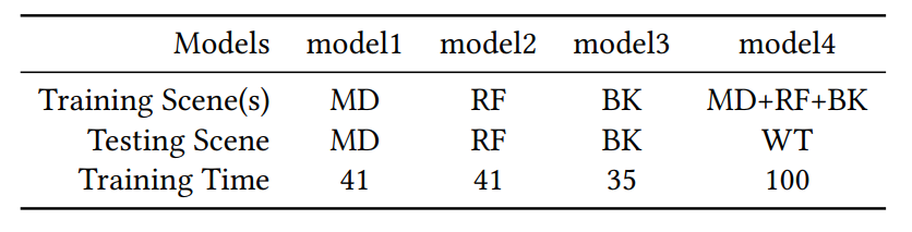
Training setups and time
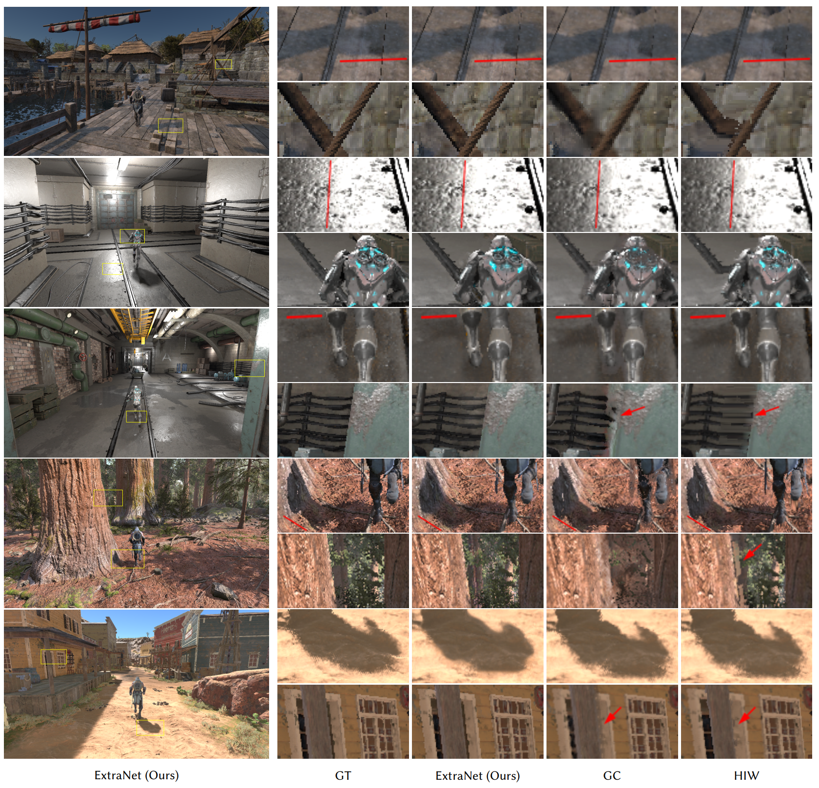
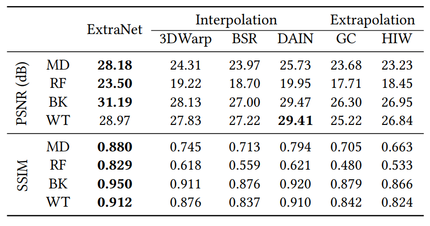
6.1. Comparisons against Frame Interpolation Methods

6.2. Comparisons against Frame Extrapolation Methods
6.3. Comparisons against ASW Technology

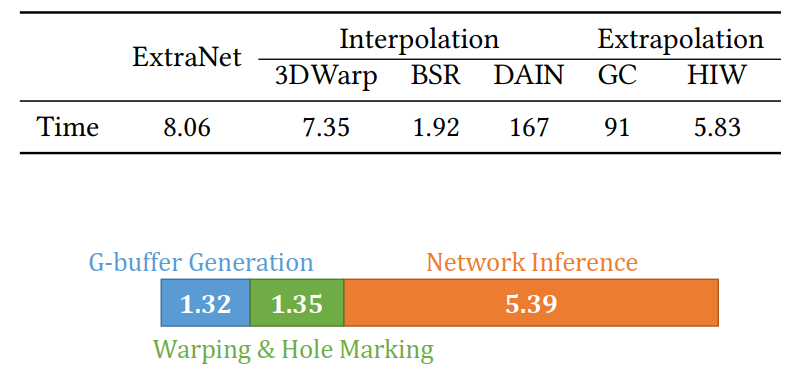
6.4. Analysis of Runtime Performance and Latency
6.5. Ablation Study
Validation of History Encoder
Validation of occlusion motion vectors

Validation of the shading-augmented loss
Failure cases


